Research · Independent project

Anisotropic Spalart–Allmaras in OpenFOAM

Updated 2026-08-26

Problem

Linear eddy-viscosity RANS models, Spalart–Allmaras included, cannot represent normal-stress anisotropy. In a straight duct they predict exactly zero turbulence-driven secondary flow, a flow feature real hardware meets everywhere.

Approach

Implement an anisotropic extension of the Spalart–Allmaras model as a custom OpenFOAM turbulence model (clean-room, from the published literature), verified from the baseline up: stock SA first, against reference data, before any model change.

Results

Baselines verified on the flat plate and channel flow; the anisotropic extension is implemented as a custom OpenFOAM model, reproduces the DNS ordering of the normal Reynolds stresses, and drives square-duct secondary flow at 1.3% of bulk (DNS: ≈2%) where stock SA gives machine zero.

Why this project

In my Cranfield group design project, supervised by László Könözsy, we investigated his anisotropic Reynolds-stress hypothesis — a unification of the Boussinesq approach with a stochastic turbulence model, previously applied to pipe flow with k–ω SST — in fully developed channel flow at Re_τ = 180 against DNS data. Each group member adapted the hypothesis to a different baseline turbulence model as an ANSYS Fluent user-defined function; my extension was to the Spalart–Allmaras model. This project rebuilds that line of work independently in OpenFOAM, from the published literature alone, so the model can live in an open toolchain and be validated in the open.

The payoff case is deliberately unforgiving. Turbulence-driven secondary flow in a square duct is weak — about 1–2% of the bulk velocity — but it redistributes wall shear stress and heat transfer, and a linear eddy-viscosity model gives literally none of it. Any secondary flow the extended model produces is signal, and DNS data exists to judge it against.

Setup

OpenFOAM v2606simpleFoam, stock Spalart–Allmaras

Flat plate, Re_L = 5×10⁶NASA TMR practice: ν̃_∞ = 3ν, plate length 2

47k cells, y⁺ ≤ 0.32wall-resolved structured mesh, graded 60,000:1

< 6 minconverged serial on an M1 Pro laptop

Baseline verification: flat plate vs NASA TMR

Before touching the turbulence model, the solver and setup have to be trusted. Following the NASA Turbulence Modeling Resource flat-plate practice, stock Spalart–Allmaras is run wall-resolved and compared against the Kármán–Schoenherr skin-friction correlation and the Coles/van Driest velocity law. Skin friction converges onto the correlation as the boundary layer develops — within 1.3% at Re_θ = 10,000, with the expected shortfall near the leading edge where the correlation assumes a fully turbulent origin. The velocity profile at Re_θ ≈ 10,000 follows the law of the wall through the sublayer, buffer layer and log layer (RMS deviation 0.19 u⁺ units in the log layer) with a healthy wake.

Flat-plate baseline, stock Spalart–Allmaras. Left: skin friction vs Re_θ against the Kármán–Schoenherr correlation (symbols) — −1.3% at Re_θ = 10,000. Right: velocity profile at Re_θ = 9,981 against the Coles/van Driest law (symbols). Reference data from the NASA Turbulence Modeling Resource.

The anisotropic extension, implemented

The extension is implemented as a custom OpenFOAM turbulence model, SpalartAllmarasAniso, compiled as a user library against OpenFOAM v2606. The closure follows Könözsy’s hypothesis — the Reynolds stress as the Boussinesq part plus a weighted anisotropic term μ_ΘΘG, where G is Czibere’s transformed similarity tensor built from the local velocity and vorticity directions — reconstructed entirely from the open literature: Czibere’s stochastic-model papers, the free front matter of Könözsy’s Springer volumes, and two open-access Cranfield theses that restate the full closure and its constants. Coupling to the one-equation SA model uses the eddy-viscosity form of the dominant shear stress, Θ = ν_t|∇×U|, which requires no turbulent-kinetic-energy transport equation; the anisotropic stress divergence enters the momentum equation and the nuTilda transport equation is left untouched. Before any physics was added, the renamed model was verified to reproduce stock Spalart–Allmaras to the last byte, so every difference below is attributable to the anisotropic terms alone.

In fully developed channel flow at Re_τ = 180 — the configuration of my original group project — both models sit on the Moser–Kim–Mansour DNS mean-velocity profile, and the friction Reynolds numbers land within 1% of the DNS value (176.8 stock, 176.4 anisotropic, vs 178.1). The anisotropy appears where it should: recovering the individual normal stresses through Czibere’s stress reconstruction splits the isotropic ⅔k of a linear eddy-viscosity model into ⟨u′u′⟩ > ⟨w′w′⟩ > ⟨v′v′⟩ — the correct DNS ordering — even with the published similarity constants and no calibration. Fitting the three λ* scale factors against the DNS over the log region (y⁺ = 60–150), as the closure prescribes, gives λ* = (2.16, 1.58, 2.20) and puts the streamwise stress on the DNS through the log layer with all three components within ≈8% at y⁺ = 100. Below y⁺ ≈ 50 the constant factors misallocate the anisotropy — consistent with the published guidance that the near-wall region requires separate calibration.

Two plots for turbulent channel flow at friction Reynolds number 180: mean velocity profiles of stock and anisotropic Spalart-Allmaras lying on the DNS data, and normal Reynolds stresses showing the anisotropic model splitting the isotropic two-thirds-k into the correct DNS ordering of streamwise, spanwise and wall-normal components. — **Channel flow, Re_τ = 180.** Left: mean velocity against the Moser–Kim–Mansour DNS (symbols) — stock and anisotropic SA overlap on this measure. Right: normal Reynolds stresses recovered via Czibere’s stress reconstruction (Θ = a₁k, Bradshaw constant a₁ = 0.3, SA’s built-in k estimate) with λ* = (2.16, 1.58, 2.20) fitted over y⁺ = 60–150, compared against the DNS (symbols); the dashed line is the isotropic ⅔k a linear eddy-viscosity model implies. The uncalibrated closure (λ* = 1) already captures the ordering; the fit sets the magnitudes in the log region.

The payoff case: square-duct secondary flow

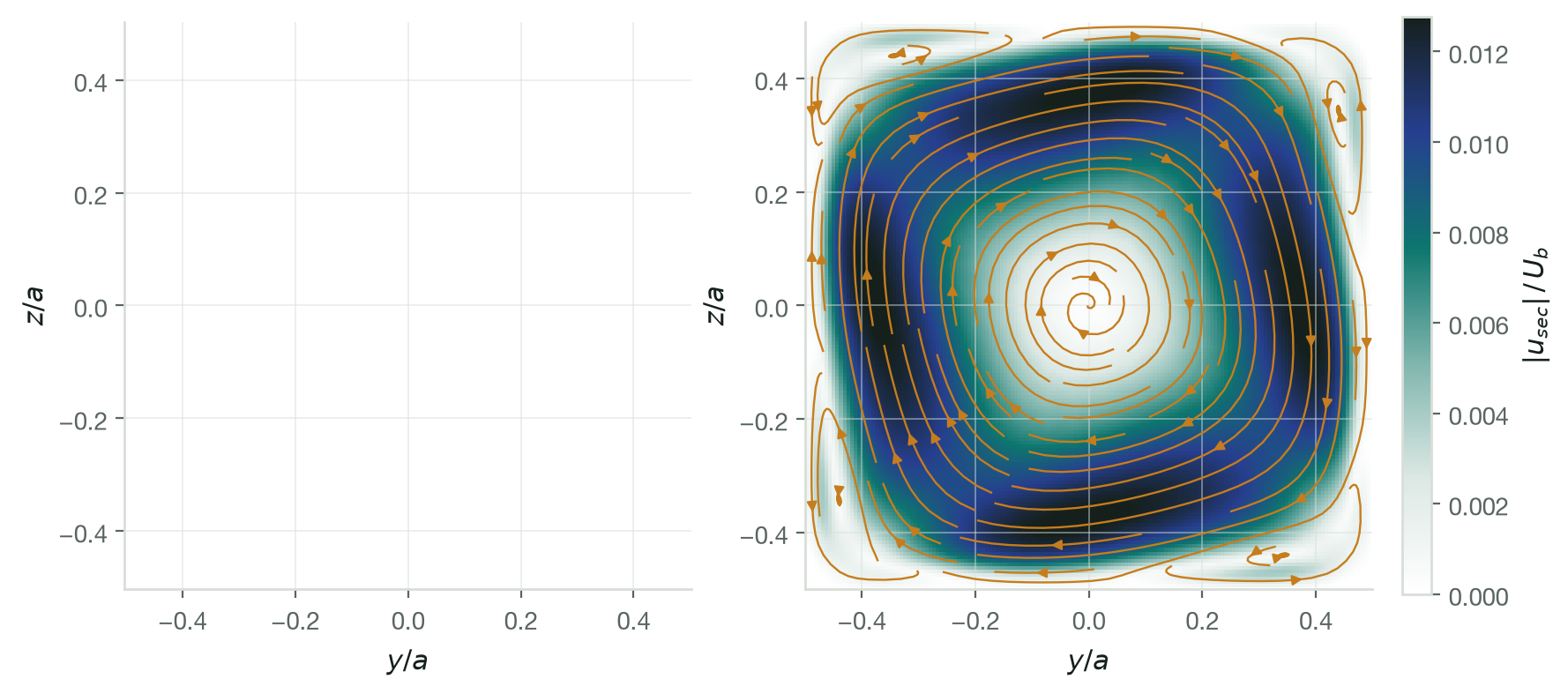
Fully developed flow in a square duct at Gavrilakis’s Re = 4410, wall-resolved over the full cross-section. Stock Spalart–Allmaras delivers its structural verdict exactly as theory says it must: the maximum cross-plane velocity is 5×10⁻¹⁴ of the bulk — machine zero. The anisotropic term breaks that degeneracy. At the default weight (μ_Θ = −0.025) a genuine secondary flow appears at 0.04% of the bulk velocity; a single calibration of the weight to μ_Θ = −0.5 raises it to 1.3%, the same order as the DNS value of roughly 2%.

The honest caveat is the topology: at these constants the model drives one coherent duct-scale rotation with small corner cells, not the eight symmetric corner vortices of the DNS. That is traceable to the fixed off-diagonal similarity constants (μ_CZ, θ_CZ, calibrated on pipe flow), which impose a preferred handedness that the duct’s symmetry should forbid. Rerunning the duct with the channel-fitted λ* factors changes neither the topology nor the magnitude appreciably (1.35% vs 1.31% of bulk) — direct evidence that the off-diagonal constants, not the diagonal scale factors, control the vortex pattern, and a concrete, well-posed target for the similarity-constant calibration this closure anticipates.

Two square cross-sections of a duct: the stock Spalart-Allmaras panel is entirely blank because its secondary flow is machine zero, while the anisotropic model panel shows cross-plane streamlines forming a duct-scale swirl with corner cells, with secondary speeds up to 1.3 percent of the bulk velocity. — **Square duct, Re = 4410 — cross-plane secondary flow.** Left: stock Spalart–Allmaras — the panel is blank because the secondary velocity is 5×10⁻¹⁴ of the bulk, i.e. machine zero. Right: anisotropic SA at μ_Θ = −0.5 — streamlines over the secondary-speed field; maximum 1.3% of bulk (DNS: ≈2%, Gavrilakis 1992). Default constants otherwise (λ* = 1).

What the flow looks like

Velocity field of the developing turbulent boundary layer on the flat plate, plotted on a logarithmic wall-normal axis, with the boundary-layer edge marked by a dashed amber line. — **The developing boundary layer.** Velocity magnitude over the plate on a logarithmic wall-normal axis — sublayer at the bottom, log layer through the mid-band, freestream above — with the δ₉₉ edge dashed. Rendered from this case’s own solution field.

Limitations, honestly

The flat-plate baseline is verification against a correlation and a composite law, not experimental data, and its near-leading-edge region sits below the Kármán–Schoenherr curve, as expected for a simulation with a genuine development region. The anisotropic results use the published similarity constants with uncalibrated scale factors (λ* = 1): the channel normal-stress ordering is captured but the near-wall streamwise peak is underestimated, and the stress recovery leans on SA’s approximate built-in k estimate. In the duct, the secondary-flow magnitude was matched to DNS order by calibrating the single weight μ_Θ, but the vortex topology does not reproduce the DNS’s eight-fold symmetric pattern — the fixed pipe-calibrated off-diagonal similarity constants impose a preferred swirl direction. No claim of predictive superiority over the baseline is made.

References

P. R. Spalart & S. R. Allmaras, A one-equation turbulence model for aerodynamic flows, La Recherche Aérospatiale 1 (1994).
L. Könözsy, A New Hypothesis on the Anisotropic Reynolds Stress Tensor for Turbulent Flows, Vols. I & II, Springer (2019, 2021) — the anisotropic framework this project builds on.
T. Czibere, Three dimensional stochastic model of turbulence, J. Comput. Appl. Mech. 2(1) (2001); and Calculating turbulent flows based on a stochastic model, J. Comput. Appl. Mech. 7(2) (2006) — the similarity theory underlying the closure.
R. D. Moser, J. Kim & N. N. Mansour, Direct numerical simulation of turbulent channel flow up to Re_τ = 590, Phys. Fluids 11 (1999) — channel reference data.
NASA Langley Turbulence Modeling Resource — flat-plate verification case and reference data (tmbwg.github.io/turbmodels).
J. Bardina, P. Huang & T. Coakley, Turbulence Modeling Validation, Testing, and Development, NASA TM 110446 (1997) — source of the Coles/van Driest composite law.
S. Gavrilakis, Numerical simulation of low-Reynolds-number turbulent flow through a straight square duct, J. Fluid Mech. 244 (1992).