Research · Independent project
A DNS→LES hybrid testbed on Xcompact3d
Subgrid models for LES are usually judged against DNS produced elsewhere, with different numerics. A DNS–LES hybrid needs both fidelities in one solver, sharing one discretisation, so that differences come from modelling — not numerics.
Build a controlled two-fidelity environment on the open-source Xcompact3d solver: DNS validated against reference data, explicit filtering for a priori subgrid testing, matched LES on the same grid family, and a DNS→LES handoff that restarts the coarse LES from the spectrally restricted DNS state.
DNS validated with grid convergence (peak dissipation −1.2% on the 129³ grid); a priori subgrid analysis of the DNS fields (27% backscatter, Smagorinsky pointwise correlation 0.22); matched 33³ LES within 2% of the reference peak decay rate; and a DNS→LES handoff after the dissipation peak that cuts the spread between subgrid models from 15 to 1.7 percentage points of final kinetic energy.
Why this project
During my master’s I modelled turbulent flame kernels with the DNS code SENGA. The ideal outcome of that work — a hybrid DNS–LES treatment, with DNS reserved for where resolving every scale matters (the growing flame kernel and its front) and LES wherever a filtered or iLES description suffices — was out of reach in the time available, largely because hybridisation needs a code you can take apart and rebuild fidelity by fidelity. This project builds that capability independently, on open tools, as a DNS→LES pathway: validated DNS first, LES built on top of it, with each step validated before the next one begins.
The vehicle is Xcompact3d, a BSD-licensed high-order finite-difference solver built for turbulence research. It is compact enough to modify deeply, and ships with canonical cases and reference data that make honest validation straightforward.
Setup
Validation: Taylor–Green vortex at Re = 1600
The Taylor–Green vortex is the standard first test for a DNS platform: a smooth initial vortex transitions to turbulence and decays, and the kinetic-energy dissipation history is acutely sensitive to both the numerics and the resolution. Both grids closely track the reference kinetic-energy decay. On the 65³ grid the dissipation peak at t ≈ 9 comes in 4.3% low — the classic signature of marginally resolved smallest scales; on the 129³ grid the peak error closes to −1.2% and the RMS deviation drops to 0.75% of peak, converging cleanly toward the reference.

What the flow looks like

A priori: testing the Smagorinsky closure against the DNS
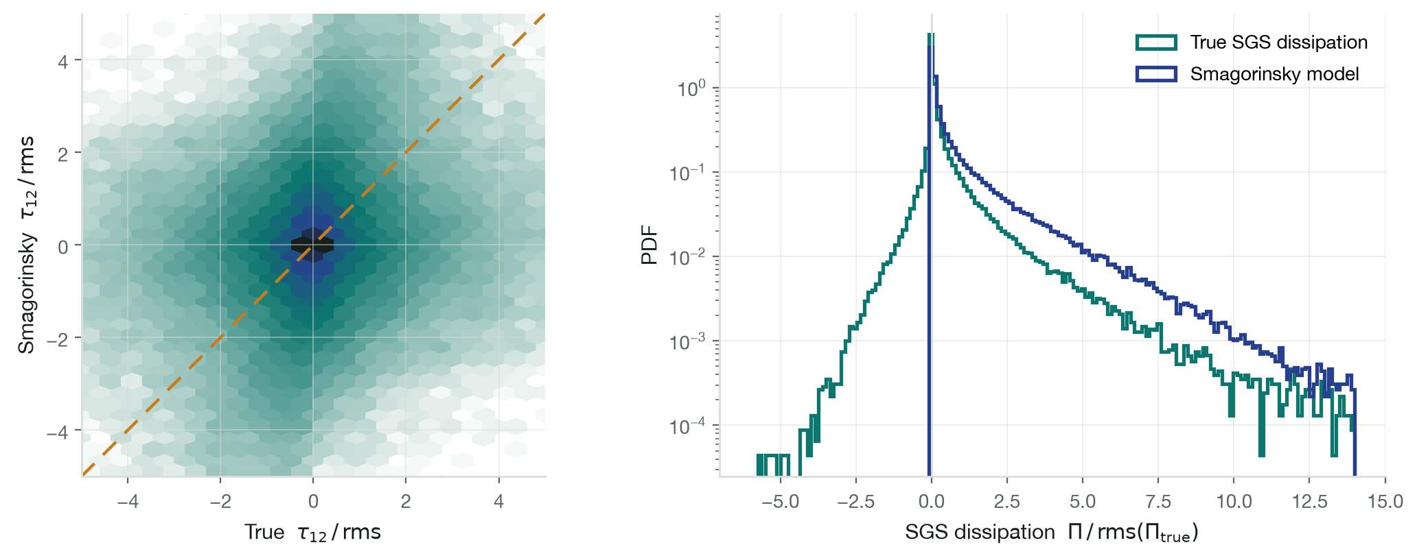
With a validated DNS in hand, the platform’s first modelling question is a priori: filter the DNS fields explicitly and ask how well a subgrid model reproduces the true subgrid stress. The t = 10 field of the 129³ simulation is filtered with a top-hat filter of width 4Δx, the exact subgrid stress τij is computed from the definition, and the static Smagorinsky prediction is evaluated from the filtered strain field.
The results reproduce the classic findings of a priori testing. Pointwise, the Smagorinsky stress correlates weakly with the truth (correlation 0.22 for τ12, 0.23 pooled over components) — the model is a poor local predictor. Energetically it does much better: the subgrid dissipation correlates at 0.75. And 27% of all points transfer energy from small scales to large (backscatter), a physical pathway an eddy-viscosity closure cannot represent at all — visible below as the negative tail the model PDF simply cuts off. Matching the mean subgrid dissipation yields Cs = 0.10 for this flow and filter scale, well below the Cs ≈ 0.17 of Lilly’s classical analysis.
A posteriori: matched LES on the same platform
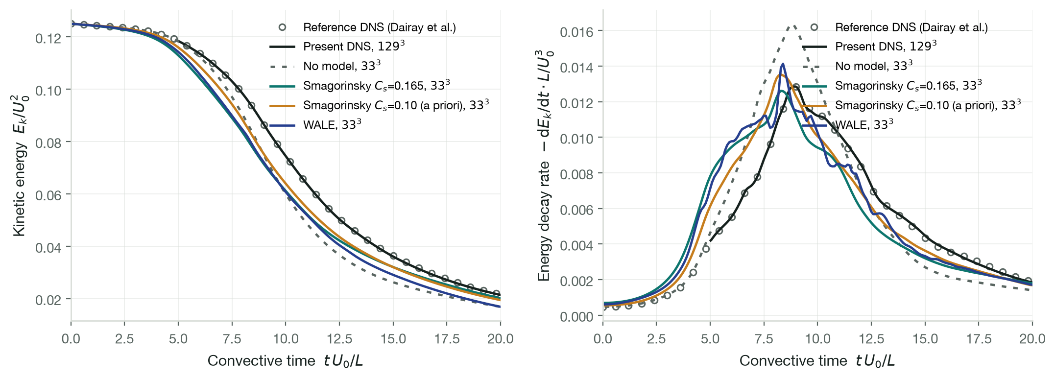
The a posteriori counterpart runs actual LES of the same flow, in the same code with the same numerics, on a 33³ grid — a quarter of the DNS resolution per direction. Four variants are compared on the total kinetic-energy decay rate, which includes the subgrid contribution: no model, classic Smagorinsky at Cs = 0.165, Smagorinsky at the a priori-matched Cs = 0.10, and WALE.
Without a model, the coarse grid piles up energy at the smallest resolved scales and overshoots the peak decay rate by 27%. Every subgrid model repairs this: Smagorinsky at Cs = 0.165 lands within −1.9% of the reference peak, the a priori constant gives +5.2%, and WALE +9.9%. The instructive part is that the a priori-matched constant does not perform best a posteriori — the well-known gap between the two testing modes, here reproduced end-to-end within a single solver, which is precisely the capability this platform was built to provide.
Blending in time: a DNS→LES handoff
The hybrid concept this platform builds toward allocates fidelity by the physics: DNS where resolving every scale matters, LES where a filtered description is enough. The Taylor–Green vortex is statistically homogeneous, so there is no spatial region to which DNS could be confined — but the allocation exists in time. Transition and the dissipation peak (t ≈ 9) generate the smallest scales and demand full resolution; the self-similar decay afterwards does not. The handoff runs DNS through the peak, then restarts the 33³ LES from the DNS state and lets it carry the decay.
Two pieces of machinery make this work. A small solver extension reads an arbitrary initial velocity field into the TGV case (double-precision, through the code’s own parallel IO). And the transfer itself is a sharp spectral restriction of the 129³ snapshot onto the 33³ grid — cosine/sine transforms matched to each velocity component’s parity under the free-slip boundaries, truncated at the coarse grid’s resolution limit, with a machine-precision round-trip self-test. The distinction matters: top-hat filtering followed by point sampling aliases the surviving subfilter energy onto the coarse grid, and in a first attempt the numerics burned off 42% of the kinetic energy within a fraction of a time unit. The spectral restriction transfers 99.2% of the DNS kinetic energy and the continuation is immediately stable, the projection step absorbing the small divergence the coarse discretisation sees.
Handing off after the peak (th = 10), all three coarse-grid variants — no model, Smagorinsky Cs = 0.165, WALE — track the reference decay to within 6.4–7.3% RMS of the peak decay rate and finish at t = 20 within −7.1% to −8.8% of the reference kinetic energy: a spread of just 1.7 percentage points across models. The same three models run from t = 0 span −6.5% to −21.8% — a 15-point spread. Starting from the true resolved state removes the error a from-scratch LES accumulates through transition, and with it most of the sensitivity to the subgrid model. The eddy-viscosity models do over-dissipate for about one time unit after the handoff while adjusting to the sharply truncated spectrum (Smagorinsky most, visible as the spike at th); the quoted decay-rate statistics exclude that adjustment window.
Handing off before the peak (th = 7.5) is the ablation that justifies the allocation. Even with the spectrally exact transfer, the 33³ grid cannot produce the peak: all three variants overshoot it by 21–34% and mistime it, because the peak’s physics lives partly in the scales the coarse grid cannot hold. The peak belongs to DNS; the decay does not — which is the hybrid argument in one figure.
How early is too early depends on the LES resolution — the allocation boundary moves. Repeating the pre-peak handoff on a 65³ grid, half the DNS resolution, the no-model continuation captures the peak within +5.3% with the timing right and finishes at t = 20 within +0.8% of the reference energy; WALE gives +11.6% on the peak. At this resolution the truncated band carries so little of the motion that added eddy viscosity mostly over-damps — where the grid is fine enough, the implicit route suffices, and where it is not, no subgrid model rescues the peak. Choosing the handoff time is therefore a resolution-versus-cost trade the platform can now measure directly.
The cost asymmetry is what makes the handoff worth having: on the same 8 MPI ranks, the measured wall time of the 129³ DNS is ≈172 s per convective time unit against ≈21 s for the 33³ LES leg — the decay half of the simulation for an eighth of the price.

Limitations, honestly
One canonical case, and the comparison target is the reference dataset shipped with Xcompact3d itself — a strong but in-family benchmark. The a priori analysis uses a single snapshot (t = 10) and a single filter width (4Δx) with reflected boundaries on the symmetric sub-box; the a posteriori decay rates are finite-differenced from the recorded kinetic energy. The a priori-matched constant was obtained at the DNS filter scale, not the 33³ LES grid scale — part of why it does not transfer directly. The handoff presented here blends the two fidelities in time, which is the split this homogeneous flow admits; a spatially zonal coupling — DNS embedded in an LES domain with a resolved interface — is a different and harder problem, and is not attempted. The handoff’s decay-rate statistics exclude the one-unit model adjustment window after th, stated as such above.
References
- P. Bartholomew et al., Xcompact3d: An open-source framework for solving turbulence problems on a Cartesian mesh, SoftwareX 12 (2020).
- S. Laizet & E. Lamballais, High-order compact schemes for incompressible flows: A simple and efficient method with quasi-spectral accuracy, J. Comput. Phys. 228 (2009).
- M. Brachet et al., Small-scale structure of the Taylor–Green vortex, J. Fluid Mech. 130 (1983).
- T. Dairay, E. Lamballais, S. Laizet & J. C. Vassilicos, Numerical dissipation vs. subgrid-scale modelling for large eddy simulation, J. Comput. Phys. 337 (2017) — source paper for the reference dataset.
- J. Smagorinsky, General circulation experiments with the primitive equations, Mon. Weather Rev. 91 (1963).
- F. Nicoud & F. Ducros, Subgrid-scale stress modelling based on the square of the velocity gradient tensor, Flow Turbul. Combust. 62 (1999).
- R. A. Clark, J. H. Ferziger & W. C. Reynolds, Evaluation of subgrid-scale models using an accurately simulated turbulent flow, J. Fluid Mech. 91 (1979).
- Reference data: TGV Re = 1600 statistics distributed with Xcompact3d (Dairay et al. 2017 DNS, 512³ over the full box; data file dated 2018).